Building Custom Ion Channels from Scratch

In Example 1, we used GateSpec and GenericChannel to build a Hodgkin-Huxley neuron in just a few lines of code. But what if you need a channel that doesn't fit the standard alpha/beta gating paradigm? What if you want to implement a complex Markov chain model, or non-standard biophysics?

GenericChannel isn't a black box—it's just a convenience wrapper around standard ModelingToolkit components.

The only rule for an ion channel in this toolkit is that it must be an MTK system that extends a standard electrical OnePort. Let's prove it by building a custom leak channel and a custom persistent sodium channel (NaP) from first principles.

using MTKNeuralToolkit
using ModelingToolkit: mtkcompile, @named, @variables, @parameters, t_nounits as t, D_nounits as D, extend, @component, @unpack, System
using ModelingToolkitStandardLibrary.Electrical: OnePort
using OrdinaryDiffEq
using Plots

1. A Custom Leak Channel

A leak channel has no states; it simply follows Ohm's law:

\[I = g(V - E)\]

We define it as an MTK @component that wraps an OnePort. The steps are:

1. Instantiate the OnePort to get the voltage v and current i.
2. Define parameters g and E_rev.
3. Write the governing equation.
4. Extend the OnePort with our equations. This tells MTK that our component behaves as an electrical OnePort, which is exactly what build_compartment expects.

@component function CustomLeakChannel(; name, g=0.3, E_rev=-54.4)
    @named oneport = OnePort()
    @unpack v, i = oneport
    @parameters g=g E_rev=E_rev
    eqs = [i ~ g * (v - E_rev)]
    return extend(System(eqs, t, [], [g, E_rev]; name=name), oneport)
end

CustomLeakChannel (generic function with 1 method)

2. A Custom Persistent Sodium Channel (NaP)

Let's build a channel with a single gating variable, m, that does not inactivate (persistent). We'll use a custom steady-state function and a time constant, writing out the ODE manually.

The gating ODE is:

\[\frac{dm}{dt} = \frac{m_{\infty} - m}{\tau}\]

And the current equation is:

\[I = g \cdot m^p \cdot (V - E)\]

Let's use $p=1$ for NaP. We initialize the state variable m based on V_init.

@component function CustomNaPChannel(; name, g=10.0, E_rev=50.0, V_init=-65.0)
    @named oneport = OnePort()
    @unpack v, i = oneport

    @parameters g=g E_rev=E_rev
    @variables m(t) = 1.0 / (1.0 + exp(-(V_init + 50.0) / 5.0))

    m_inf(V) = 1.0 / (1.0 + exp(-(V + 50.0) / 5.0))
    tau_m = 5.0

    eqs = [
        D(m) ~ (m_inf(v) - m) / tau_m,
        i ~ g * m * (v - E_rev)
    ]

    return extend(System(eqs, t, [m], [g, E_rev]; name=name), oneport)
end

CustomNaPChannel (generic function with 1 method)

3. Assemble the Compartment

We instantiate our custom channels and a standard Capacitor. Note that build_compartment doesn't know or care that these are custom; it just connects their positive pins to the membrane voltage and grounds the negative pins.

top = Scalar() # Define a scalar topology

@named cap = Capacitor(topology=top, C=1.0)
@named leak = CustomLeakChannel()
@named nap = CustomNaPChannel()

Model nap:
Subsystems (2): see hierarchy(nap)
  p
  n
Equations (7):
  5 standard: see equations(nap)
  2 connecting: see equations(expand_connections(nap))
Unknowns (7): see unknowns(nap)
  v(t)
  i(t)
  m(t)
  p₊v(t)
  ⋮
Parameters (2): see parameters(nap)
  g
  E_rev

build_compartment handles the wiring just like in Example 1.

channels = [leak, nap]
soma = build_compartment(cap, channels; name=:soma, V_init=-65.0, topology=top)

Compartment{NoMorphology, NoGeometry, Float64}(Model soma:
Subsystems (7): see hierarchy(soma)
  cap
  injector
  syn_injector
  p
  ⋮
Equations (38):
  24 standard: see equations(soma)
  14 connecting: see equations(expand_connections(soma))
Unknowns (37): see unknowns(soma)
  cap₊v(t)
  cap₊i(t)
  cap₊p₊v(t)
  cap₊p₊i(t)
  ⋮
Parameters (5): see parameters(soma)
  cap₊C
  leak₊g
  leak₊E_rev
  nap₊g
  ⋮, (V = soma₊cap₊v(t), p_pin = Model soma₊p:
Equations (2):
  2 connecting: see equations(expand_connections(soma₊p))
Unknowns (2): see unknowns(soma₊p)
  v(t)
  i(t), n_pin = Model soma₊n:
Equations (2):
  2 connecting: see equations(expand_connections(soma₊n))
Unknowns (2): see unknowns(soma₊n)
  v(t)
  i(t), I_ext = soma₊injector₊I₊u(t), I_syn = soma₊syn_injector₊I₊u(t), cap_name = :cap), -65.0, Scalar(), NoGeometry(), NoMorphology())

4. Build and Simulate

We'll inject a small current to see how the persistent sodium channel interacts with the leak channel to create a steady depolarized state.

drivers = [(1, 2.0)]
net = build_acausal_network([soma]; drivers=drivers, name=:custom_neuron)

println("Compiling custom channel neuron...")
sys = mtkcompile(net.sys)
prob = ODEProblem(sys, [], (0.0, 100.0))

println("Solving...")
sol = solve(prob, Rosenbrock23(), reltol=1e-4, abstol=1e-4)

retcode: Success
Interpolation: specialized 2nd order "free" stiffness-aware interpolation
t: 88-element Vector{Float64}:
   0.0
   0.0012501739956439345
   0.0206097032318029
   0.039969232467961864
   0.07556096691783404
   0.1111527013677062
   0.1566873295232779
   0.2022219576788496
   0.2504812464902859
   0.29874053530172223
   ⋮
  24.037970853133118
  27.101561326850348
  30.79717890558891
  35.40393491713189
  41.42992427012772
  49.92628954411219
  63.581814207884044
  92.89418038495506
 100.0
u: 88-element Vector{Vector{Float64}}:
 [0.04742587317756678, -65.0]
 [0.04742595775449338, -64.9253759854762]
 [0.04744999458832616, -63.77872780373131]
 [0.047523430450827145, -62.648088859189684]
 [0.0478182385814619, -60.60622915203647]
 [0.04838558103120771, -58.60357151857695]
 [0.049644871828944365, -56.078102419476274]
 [0.05169733952103672, -53.56458037326817]
 [0.05495463633770272, -50.87155271266383]
 [0.059474246020049276, -48.10165443439661]
 ⋮
 [0.991920007130865, 47.13043887694605]
 [0.9956658744873588, 47.14112828735096]
 [0.9979678705076583, 47.147658057687764]
 [0.9992207322125657, 47.151199540938194]
 [0.9997868150979198, 47.152796913319534]
 [0.9999718520633931, 47.153318693587146]
 [1.0000011366539605, 47.15340126116649]
 [0.9999997757415475, 47.153397426401874]
 [0.9999999511145985, 47.153397920671985]

5. Plot the Results

We can access the variables of our custom components exactly as we would with the pre-built channels, reaching into the compiled system's namespace.

p1 = plot(sol, idxs=[sys.soma.cap.v],
          title="Example 0: Custom Channel Voltage",
          ylabel="V (mV)", legend=false)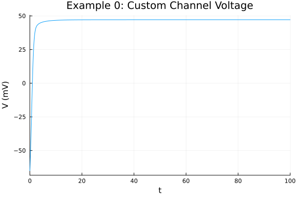

Look at the gating variable m of our custom NaP channel!

p2 = plot(sol, idxs=[sys.soma.nap.m],
          title="Custom NaP Gating Variable (m)",
          ylabel="Fraction open", xlabel="Time (ms)", legend=false)

plot(p1, p2, layout=(2,1), size=(800, 600))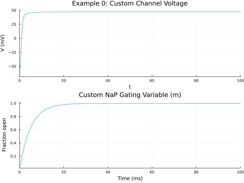

OK... nobody said it was going to be an interesting channel!

This page was generated using Literate.jl.