12. Parameter Estimation: Single Neuron

Introduction

In this example, we demonstrate the filtering power of the Prediction Error Method (PEM). We generate data from a true Hodgkin-Huxley neuron, add Gaussian noise to the voltage trace, and then attempt to recover the conductances. The PEM observer channel acts like a fixed gain Kalman Filter, absorbing the noise while allowing the optimiser to find the true underlying parameters without overfitting the noise.

using MTKNeuralToolkit
using SymbolicIndexingInterface: getu
using MTKNeuralToolkit.HodgkinHuxley: SodiumChannel, PotassiumChannel, LeakChannel
using ModelingToolkit: mtkcompile, @named
using OrdinaryDiffEq
using OrdinaryDiffEqRosenbrock
using Optimization
using OptimizationOptimJL
using SciMLStructures: Tunable, canonicalize, replace
using SymbolicIndexingInterface: parameter_values, setp
using PreallocationTools
using DataInterpolations
using SciMLBase
using Plots
using Markdown
using Random

1. Build the True System & Generate Noisy Data

top = Scalar()

function build_hh_neuron(name::Symbol; gNa=120.0, gK=36.0, gleak=0.3, pem=false, itps=nothing, K=1.0)
    @named cap  = Capacitor(topology=top, C=1.0)
    @named na   = SodiumChannel(topology=top, g=gNa)
    @named k    = PotassiumChannel(topology=top, g=gK)
    @named leak = LeakChannel(topology=top, g=gleak)
    channels = [na, k, leak]
    if pem
        @named pem_ch = PEMObservationChannel(itps=itps, K_init=K, topology=top)
        push!(channels, pem_ch)
    end
    return build_compartment(cap, channels; name=name, V_init=-65.0, topology=top)
end

true_gNa = 120.0
true_gK  = 36.0
true_gleak = 0.3

true_neuron = build_hh_neuron(:true_neuron; gNa=true_gNa, gK=true_gK, gleak=true_gleak)

drivers = [(1, 8.0)]
true_net = build_acausal_network([true_neuron]; drivers=drivers, name=:true_net)
END_TIME= 100.0


true_sys = mtkcompile(true_net.sys)
true_prob = ODEProblem(true_sys, [], (0.0, END_TIME))
timesteps = 0.0:0.1:END_TIME

true_sol = solve(true_prob, Rodas5(); saveat=timesteps)
V_data_clean = true_sol[true_sys.true_neuron.cap.v];

Add 3 mV Gaussian noise to the data

Random.seed!(42)
noise_level = 3.0
V_data_noisy = V_data_clean .+ noise_level .* randn(length(V_data_clean))
itp_V = LinearInterpolation(V_data_noisy, timesteps);

2. Setup the PEM Optimization Problem

We create a model neuron with terrible initial guesses and attach a PEM observer to the noisy data.

guess_gNa = 10.0
guess_gK  = 100.0
guess_gleak = 10.3

fit_neuron = build_hh_neuron(:fit_neuron; gNa=guess_gNa, gK=guess_gK, gleak=guess_gleak, pem=true, itps=[itp_V], K=2.0)
fit_net = build_acausal_network([fit_neuron]; drivers=drivers, name=:fit_net)
fit_sys = mtkcompile(fit_net.sys)
fit_prob = ODEProblem(fit_sys, [], (0.0, END_TIME))

gNa_sym = fit_sys.fit_neuron.na.g
gK_sym  = fit_sys.fit_neuron.k.g
gleak_sym = fit_sys.fit_neuron.leak.g

setter = setp(fit_prob, [gNa_sym, gK_sym, gleak_sym])
diffcache = DiffCache(copy(canonicalize(Tunable(), parameter_values(fit_prob))[1]))

v_getter = getu(fit_prob, fit_sys.fit_neuron.cap.v)
i_pem_getter = getu(fit_prob, fit_sys.fit_neuron.pem_ch.i);

3. Define Loss Function & Optimize

We calculate a multi-objective loss based on both the tracking error (voltage) and the observer effort (current). This forces the system to track the data while penalizing the controller from "cheating" to force bad parameters to fit.

function loss(x, p)
    prob, timesteps, V_data_noisy, setter, diffcache, v_getter, i_pem_getter = p

    ps = parameter_values(prob)
    buffer = get_tmp(diffcache, x)
    copyto!(buffer, canonicalize(Tunable(), ps)[1])
    ps = replace(Tunable(), ps, buffer)
    setter(ps, x)
    newprob = remake(prob; p=ps)
    sol = solve(newprob, Rodas5(); saveat=timesteps, reltol=1e-8, abstol=1e-8)

    if !SciMLBase.successful_retcode(sol.retcode)
        return Inf
    end

    V_fit = v_getter(sol)
    I_pem = i_pem_getter(sol)

    #Multi-objective cost
    tracking_error = sum(abs2, V_fit .- V_data_noisy) / length(V_data_noisy)
    observer_effort = sum(abs2, I_pem) / length(I_pem)

    #Weights
    alpha = 1.0
    beta = 1.0

    return alpha * tracking_error + beta * observer_effort
end

loss (generic function with 1 method)

Tuple must also have exactly 7 items:

opt_params = (fit_prob, timesteps, V_data_noisy, setter, diffcache, v_getter, i_pem_getter)
adtype = AutoForwardDiff()
optfn = OptimizationFunction(loss, adtype)
optprob = OptimizationProblem(optfn, [guess_gNa, guess_gK, guess_gleak], opt_params)

OptimizationProblem. In-place: true
u0: 3-element Vector{Float64}:
  10.0
 100.0
  10.3

4. Optimize and Plot

To avoid recompiling new systems for the free-running simulations, we simply reuse the compiled fit_sys and set the PEM controller gain (K) to 0.0 to disable the observer.

println("Starting optimization...")
res = solve(optprob, BFGS(); maxiters=1000)

K_sym = fit_sys.fit_neuron.pem_ch.K
K_setter = setp(fit_prob, [K_sym])

SymbolicIndexingInterface.ParameterHookWrapper{SymbolicIndexingInterface.MultipleSetters{Vector{SymbolicIndexingInterface.SetParameterIndex{ModelingToolkitBase.ParameterIndex{SciMLStructures.Tunable, Int64}}}}, Vector{Symbolics.Num}}(SymbolicIndexingInterface.MultipleSetters{Vector{SymbolicIndexingInterface.SetParameterIndex{ModelingToolkitBase.ParameterIndex{SciMLStructures.Tunable, Int64}}}}(SymbolicIndexingInterface.SetParameterIndex{ModelingToolkitBase.ParameterIndex{SciMLStructures.Tunable, Int64}}[SymbolicIndexingInterface.SetParameterIndex{ModelingToolkitBase.ParameterIndex{SciMLStructures.Tunable, Int64}}(ModelingToolkitBase.ParameterIndex{SciMLStructures.Tunable, Int64}(SciMLStructures.Tunable(), 8, false))]), Symbolics.Num[fit_neuron₊pem_ch₊K])

–- 1. Simulate with recovered parameters (WITH PEM) to get observer current –-

opt_ps = parameter_values(fit_prob)
opt_buffer = copy(canonicalize(Tunable(), opt_ps)[1])
opt_ps = replace(Tunable(), opt_ps, opt_buffer)
setter(opt_ps, res.u) # set recovered parameters
opt_prob_pem = remake(fit_prob; p=opt_ps)
opt_sol_pem = solve(opt_prob_pem, Rodas5(); saveat=timesteps, reltol=1e-6, abstol=1e-6)

retcode: Success
Interpolation: 1st order linear
t: 1001-element Vector{Float64}:
   0.0
   0.1
   0.2
   0.3
   0.4
   0.5
   0.6
   0.7
   0.8
   0.9
   ⋮
  99.2
  99.3
  99.4
  99.5
  99.6
  99.7
  99.8
  99.9
 100.0
u: 1001-element Vector{Vector{Float64}}:
 [0.052, 0.596, 0.317, -65.0]
 [0.05330224258733806, 0.5958257231397336, 0.31713188917928076, -64.10495208851454]
 [0.056186658548967976, 0.5952638065465109, 0.3175247052435673, -63.28045619547058]
 [0.05969677442116969, 0.5944052124703861, 0.3181131958489684, -62.65603848551341]
 [0.06382260661121056, 0.5932300013703545, 0.31890698767163456, -61.74135768811049]
 [0.06932400701385522, 0.5915633269870064, 0.32001506698805826, -60.696519014785444]
 [0.07526597061212055, 0.5895130026642212, 0.32136052535063325, -60.19174969938137]
 [0.08005300484517525, 0.587376725400251, 0.322751031276136, -60.156235625323916]
 [0.08331498384191342, 0.5852944926743975, 0.32409805294649596, -60.29563796805962]
 [0.08576533242114168, 0.5832252000656628, 0.3254279853731604, -59.84447136636075]
 ⋮
 [0.9875191542206222, 0.14302611819542213, 0.6858944479464151, 10.865684142318866]
 [0.9868375378926052, 0.1297373827687635, 0.7017803454320481, 5.451275057477877]
 [0.9839418768342546, 0.11785432768944293, 0.7148887520928288, 0.1913368186637163]
 [0.9788936886005584, 0.10729493325520807, 0.7255766823419945, -4.834969112971681]
 [0.9714132075401531, 0.09799754731699004, 0.7341415435561855, -9.673783077707123]
 [0.9606621646038648, 0.08994319495164053, 0.7407583645712061, -14.878176801931987]
 [0.9455406223372396, 0.08314037780951977, 0.7455701577880091, -19.34966581635644]
 [0.9259617474927013, 0.07750895188876242, 0.7489131307147232, -23.805165316589722]
 [0.8997550691087185, 0.07310653932758869, 0.7508021810491343, -28.342850142202455]

–- 2. Pure simulation for INITIAL GUESS (No PEM) –-

init_ps = parameter_values(fit_prob)
init_buffer = copy(canonicalize(Tunable(), init_ps)[1])
init_ps = replace(Tunable(), init_ps, init_buffer)
setter(init_ps, [guess_gNa, guess_gK, guess_gleak])
K_setter(init_ps, [0.0]) # disable PEM controller
init_prob_free = remake(fit_prob; p=init_ps)
init_eval_sol = solve(init_prob_free, Rodas5(); saveat=timesteps)

retcode: Success
Interpolation: 1st order linear
t: 1001-element Vector{Float64}:
   0.0
   0.1
   0.2
   0.3
   0.4
   0.5
   0.6
   0.7
   0.8
   0.9
   ⋮
  99.2
  99.3
  99.4
  99.5
  99.6
  99.7
  99.8
  99.9
 100.0
u: 1001-element Vector{Vector{Float64}}:
 [0.052, 0.596, 0.317, -65.0]
 [0.061290858530422494, 0.5942952843383317, 0.318137305411624, -58.70817014124696]
 [0.07730047544215801, 0.590609742063318, 0.3204915318624678, -56.702232466545524]
 [0.09253428914116847, 0.5862459234196883, 0.32322088468856697, -56.08879527296019]
 [0.10502266115176447, 0.5817235920244812, 0.3260211377312959, -55.926509323552615]
 [0.1146688286712826, 0.577220825406562, 0.32879184097563885, -55.910557539390936]
 [0.12189796058700975, 0.5727952528923334, 0.3315011249766164, -55.94299551617634]
 [0.127203089557158, 0.5684649201604384, 0.3341393664088835, -55.99270195382879]
 [0.1310163984823134, 0.5642352991472477, 0.3367039957035816, -56.04956671005895]
 [0.13368349618210665, 0.5601076560512765, 0.3391947897373976, -56.11013491529922]
 ⋮
 [0.10648816061853868, 0.3779511514913714, 0.4151273978453165, -58.8175980514145]
 [0.10648816061768569, 0.37795114934422624, 0.41512739784167113, -58.817598051485795]
 [0.10648816061684603, 0.3779511472307147, 0.41512739783808306, -58.81759805155598]
 [0.10648816061601968, 0.37795114515082723, 0.4151273978345522, -58.81759805162506]
 [0.10648816061520663, 0.37795114310457045, 0.41512739783107855, -58.817598051693025]
 [0.1064881606144069, 0.37795114109196726, 0.4151273978276623, -58.81759805175989]
 [0.10648816061362049, 0.3779511391130565, 0.41512739782430336, -58.81759805182563]
 [0.10648816061284742, 0.37795113716789325, 0.4151273978210019, -58.817598051890265]
 [0.10648816061208773, 0.3779511352565488, 0.41512739781775804, -58.81759805195378]

–- 3. Pure simulation for RECOVERED PARAMETERS (No PEM) –-

opt_gNa, opt_gK, opt_gleak = res.u
fit_ps = parameter_values(fit_prob)
fit_buffer = copy(canonicalize(Tunable(), fit_ps)[1])
fit_ps = replace(Tunable(), fit_ps, fit_buffer)
setter(fit_ps, [opt_gNa, opt_gK, opt_gleak])

disable PEM controller

K_setter(fit_ps, [0.0])
fit_prob_free = remake(fit_prob; p=fit_ps)
fit_eval_sol = solve(fit_prob_free, Rodas5(); saveat=timesteps)

p1 = plot(timesteps, V_data_noisy, label="Noisy Target", color=:gray, lw=1, alpha=0.8)
plot!(p1, timesteps, V_data_clean, label="True Clean", color=:black, lw=2)
plot!(p1, timesteps, init_eval_sol[fit_sys.fit_neuron.cap.v], label="Initial Guess (Free-Running)", ls=:dot, lw=2, color=:blue)
plot!(p1, timesteps, fit_eval_sol[fit_sys.fit_neuron.cap.v], label="Fit (Free-Running)", ls=:dash, lw=2, color=:red)
title!("Voltage Trace Recovery (Noisy Data)")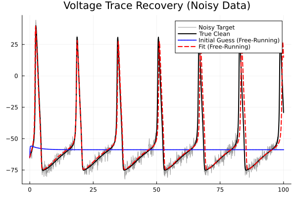

Plot the observer current.

I_obs = i_pem_getter(opt_sol_pem)
p2 = plot(timesteps, I_obs, label="Observer Current", color=:red, lw=1.5)
title!("PEM Observer Current (Absorbing Noise)")
hline!([0.0], color=:gray, ls=:dot, label="0")

p = plot(p1, p2, layout=(2,1), size=(800, 700), legend=:outertop)
xlabel!(p, "Time (ms)")
ylabel!(p, "V (mV) / I (nA)")
p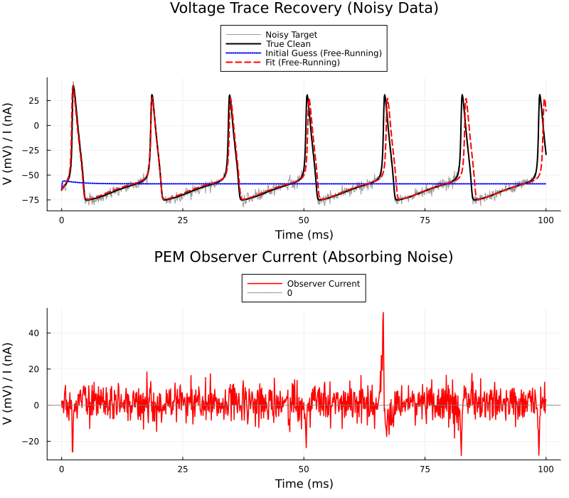

Note the slight phase lag at the end of the sim.

5. Parameter Comparison

Markdown.parse("""
| Parameter | True Value | Initial Guess | Recovered Value |
|-----------|------------|---------------|-----------------|
| gNa       | $true_gNa  | $guess_gNa    | $(round(opt_gNa, digits=3)) |
| gK        | $true_gK   | $guess_gK     | $(round(opt_gK, digits=3)) |
| gleak     | $true_gleak| $guess_gleak  | $(round(opt_gleak, digits=3)) |
""")

Parameter	True Value	Initial Guess	Recovered Value
gNa	120.0	10.0	112.119
gK	36.0	100.0	32.743
gleak	0.3	10.3	0.429

This page was generated using Literate.jl.